Low-rank matrices: using structure to recover missing data
Tensor networks are probably the most important tool in my research, and I want
explain them. Before I can do this however, I should first talk about low-rank
matrix decompositions, and why they’re so incredibly useful. At the same time I
will illustrate everything using examples in Python code, using numpy.
The singular value decomposition
Often if we have an matrix, we can write it as the product of two smaller matrices. If such a matrix has rank , then we can write it as the product of an and matrix. Equivalently, this is the number of linearly independent columns or rows the matrix has, or if we see the matrix as a linear map , then it is the dimension of the image of this linear map.
In practice we can figure out the rank of a matrix by computing its singular value decomposition (SVD). If you studied data science or statistics, then you have probably seen principal component analysis (PCA); this is very closely related to the SVD. Using the SVD we can write a matrix as a product
Where and are orthogonal matrices, and is a diagonal matrix. The values on the diagonals of are known as the singular values of . The matrices and also have nice interpretations; the rows of form an orthonormal basis of the row space of , and the columns of are an orthonormal basis of the column space of .
In numpy we can compute the SVD of a matrix using np.linalg.svd. Below we
compute it and verify that indeed :
import numpy as np

# Generate a random 10x20 matrix of rank 5
m, n, r = (10, 20, 5)
A = np.random.normal(size=(m, r))
B = np.random.normal(size=(r, n))
X = A @ B

# Compute the SVD
U, S, V = np.linalg.svd(X, full_matrices=False)

# Confirm U S V = X
np.allclose(U @ np.diag(S) @ V, X)
Output
True
Note that we called np.linalg.svd with the keyword full_matrices=False. If
left to the default value True, then in this case V would be a {20\times
20}$ matrix, as opposed to the $10\times 20 matrix it is now. Also S is
returned as a 1D array, and we can convert it to a diagonal matrix using
np.diag. Finally the function np.allclose checks if all the entries of two
matrices are almost the same; they never will be exactly the same due to
numerical error.
As mentioned before, we can use the singular values S to determine what the
rank is the matrix X. This is obvious if we plot the singular values:
import matplotlib.pyplot as plt

DEFAULT_FIGSIZE = (8, 5)

plt.figure(figsize=DEFAULT_FIGSIZE)

plt.plot(np.arange(1, len(S) + 1), S, "o")
plt.xticks(np.arange(1, len(S) + 1))
plt.yscale("log")
plt.title("Plot of singular values")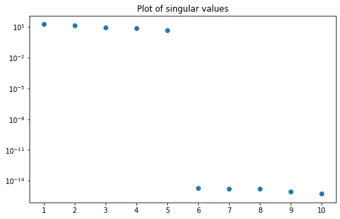
We see that the first 5 singular values are roughly the same size, but that the last five singular values are much smaller; on the order of the machine epsilon.
Knowing the matrix is rank 5, can we write it as the product of two rank 5
matrices? Absolutely! And we do this using the SVD, or rather the truncated
singular value decomposition. Since the last 5 values of S are very close to
zero, we can simply ignore them. This then means dropping the last 5 columns of
U and the last 5 rows of V. Then finally we just need to ‘absorb’ the
singular values into one of the two matrices U or V, This way we write X
as the product of a and matrix.
A = U[:, :r] * S[:r]
B = V[:r, :]
print(A.shape, B.shape)

np.allclose(A @ B, X)
Output
(10, 5) (5, 20)
True
SVD as data compression method
We rarely encounter real-world data that can be exactly represented by a low rank matrix using the truncated SVD. But we can still use the truncated SVD to get a good approximation of the data.
Let us look at the singular values of an image of the St. Vitus church in my hometown. Note that a black-and-white image is really just a matrix.
from matplotlib import image

# Load and plot the St. Vitus image
plt.figure(figsize=(14, 5))
plt.subplot(1, 2, 1)
img = image.imread("vitus512.png")
img = img / np.max(img)  # make entries lie in range [0,1]
plt.imshow(img, cmap="gray")
plt.axis("off")

# Compute and plot the singular values
plt.subplot(1, 2, 2)
plt.title("Singular values")
U, S, V = np.linalg.svd(img)
plt.yscale("log")
plt.plot(S)
We see here that the first few singular values are much larger than the rest, followed by a slow decay, and then finally a sharp drop at the very end. Note that there are 512 singular values, because this is a 512x512 image.
Let’s now try to see what happens if we compress this image as a low rank matrix using the truncated singular value decomposition. We will look what happens to the image when seen as a rank 10,20,50 or 100 matrix.
plt.figure(figsize=(12, 12))
for i, rank in enumerate([10, 20, 50, 100]):
    # Compute truncated SVD
    U, S, V = np.linalg.svd(img)
    img_compressed = U[:, :rank] @ np.diag(S[:rank]) @ V[:rank, :]

    # Plot the image
    plt.subplot(2, 2, i + 1)
    plt.title(f"Rank {rank}")
    plt.imshow(img_compressed, cmap="gray")
    plt.axis("off")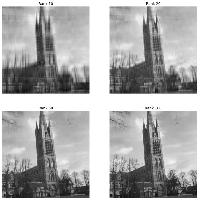
We see that even the rank 10 and 20 images are pretty recognizable, but with heavy artifacts. On the other hand the rank 50 image looks pretty good, but not as good as the original. The rank 100 image on the other hand looks really close to the original.
How big is the compression if we do this? Well, if we write the image as a rank 10 matrix, we need two 512x10 matrices to store the image, which adds up to 10240 parameters, as opposed to the original 262144 parameters; a decrease in storage of more than 25 times! On the other hand, the rank 100 image is only about 2.6 times smaller than the original. Note that this is not a good image compression algorithm; the SVD is relatively expensive to compute, and other compression algorithms can achieve higher compression ratios with less image degradation.
The conclusion we can draw from this is that we can use truncated SVD to compress data. However, not all data can be compressed as efficiently by this method. It depends on the distribution of singular values; the faster the singular values decay, the better a low rank decomposition is going to approximate our data. Images are not good examples of data that can be compressed efficiently as a low rank matrix.
One reason why it’s difficult to compress images is because they contain many sharp edges and transitions. Low rank matrices are especially bad at representing diagonal lines. For example, the identity matrix is a diagonal line seen as an image, and it is also impossible to compress using an SVD since all singular values are equal.
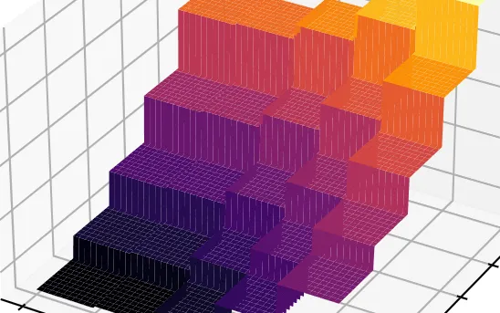
On the other hand, images without any sharp transitions can be approximated quite well using low rank matrices. These kind of images rarely appear as natural images, but rather they can be discrete representations of smooth functions . For example below we show a two-dimensional discretized sum of trigonometric functions and its singular value decomposition.
# Make a grid of 100 x 100 values between [0,1]
x = np.linspace(0, 1, 100)
y = np.linspace(0, 1, 100)
x, y = np.meshgrid(x, y)

# A smooth trigonometric function
def f(x, y):
    return np.sin(200 * x + 75 * y) + np.sin(50 * x) + np.cos(100 * y)


plt.figure(figsize=(12, 5))
plt.subplot(1, 2, 1)
X = f(x, y)
plt.imshow(X)

plt.subplot(1, 2, 2)
U, S, V = np.linalg.svd(X)
plt.plot(S)
plt.yscale("log")
plt.title("Singular values")
print(f"The matrix is approximately of rank: {np.sum(S>1e-12)}")
Output
The matrix is approximately of rank: 4
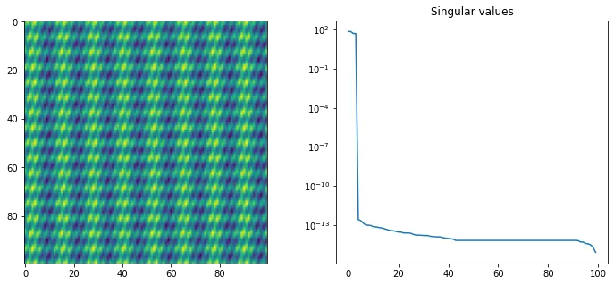
We see that this particular function can be represented by a rank 4 matrix! This is not obvious if you look at the image. In these kind of situations a low-rank matrix decomposition is much better than many image compression algorithms. In this case we can reconstruct the image using only 8% of the parameters. (Although more advanced image compression algorithms are based on wavelets, and will actually compress this very well.)
Matrix completion
Recall that a low rank matrix approximation can require much less parameters than the dense matrix it approximates. One of the powerful things about this allows us to recover the dense matrix even in the case where we only observe a small part of the matrix. That is, if we have many missing values.
In the case above we can represent the 100x100 matrix as a product of a 100x4 and 4x100 a matrix and , which has in total 800 parameters instead of 10,000. We can actually recover this low-rank decomposition from a small subset of the big dense matrix. Suppose that we observe the entries for an index set. We can recover and by solving the following least-squares problem:
This problem is however non-convex, and not straightforward to solve. There is fortunately a trick: we can alternatively fix and then optimize and vice-versa. This is known as Alternating Least Squares (ALS) optimization, and in this case works well. If we fix , observe that the minimization problem uncouples into separate linear least squares problems for each column of :
Below we do use this approach to recover the same matrix as before using 2000 data points, and we can see it does so with a very low error:
N = 2000
n = 100
r = 4

# Sample N=2000 random indices
Omega = np.random.choice(n * n, size=N, replace=False)
Omega = np.unravel_index(Omega, X.shape)
y = X[Omega]

# Use random initialization for matrices A,B
A = np.random.normal(size=(n, r))
B = np.random.normal(size=(r, n))


def linsolve_regular(A, b, lam=1e-4):
    """Solve linear problem A@x = b with Tikhonov regularization / ridge
    regression"""
    return np.linalg.solve(A.T @ A + lam * np.eye(A.shape[1]), A.T @ b)


losses = []
for i in range(40):
    loss = np.mean(((A @ B)[Omega] - y) ** 2)
    losses.append(loss)

    # Update B
    for j in range(n):
        B[:, j] = linsolve_regular(A[Omega[0][Omega[1] == j]], y[Omega[1] == j])

    # Update A
    for i in range(n):
        A[i, :] = linsolve_regular(
            B[:, Omega[1][Omega[0] == i]].T, y[Omega[0] == i]
        )

# Plot the input image
plt.figure(figsize=(12, 12))
plt.subplot(2, 2, 1)
plt.title("Input image")
S = np.zeros((n, n))
S[Omega] = y
plt.imshow(S)

# Plot reconstructed image
plt.subplot(2, 2, 2)
plt.title("Reconstructed image")
plt.imshow(A @ B)

# Plot training loss
plt.subplot(2, 1, 2)
plt.title("Mean square error loss during training")
plt.plot(losses)
plt.yscale("log")
plt.xlabel("steps")
plt.ylabel("Mean squared error")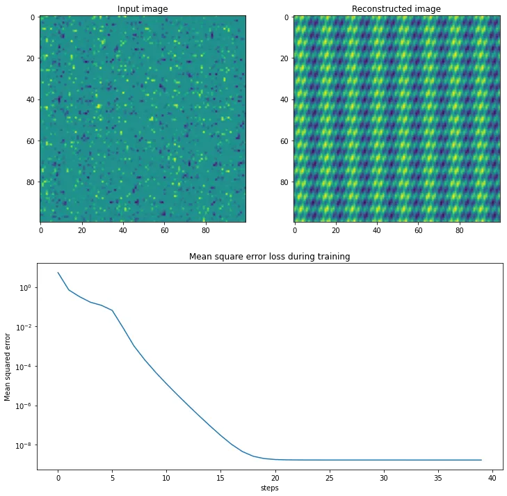
Netflix prize
Let’s consider a particularly interesting use of matrix completion — collaborative filtering. Think about how services like Netflix may recommend new shows or movies to watch. They know which movies you like, and they know which movies other people like. Netflix then recommends movies that are liked by people with a similar taste to yours. This is called collaborative filtering, because different people collaborate to filter out movies so that we can make a recommendation.
But can we do this in practice? Well, for every user we can put their personal ratings of every movie they watched in a big matrix. In this matrix each row represents a movie, and each column a user. Most users have only seen a small fraction of all the movies on the platform, so the overwhelming majority of the entries of this matrix are unknown. Then we apply matrix completion to this matrix. Each entry of the completed matrix then represents the rating we think the user would give to a movie, even if they have never watched it.
In 2006 Netflix opened a competition with a grand prize of $1,000,000 (!!) to solve precisely this problem. The data consists of more than 100 million ratings by 480,189 users for 17,769 different movies. The size of this dataset immediately poses a practical problem; if we put this in a matrix with floating point entries, then it would require about 68 terabytes of RAM. Fortunately we can avoid this problem by using sparse matrices. This makes implementation a little harder, but certainly still feasible.
We will also need to upgrade our matrix completion algorithm. The algorithm we mentioned before is slow for very large matrices, and suffers from problems of numerical stability due to the way it decouples into many smaller linear problems. Recall that complete a matrix by solving the following optimization problem:
We will first rewrite the problem as follows:
Here denotes the operation of setting all entries to zero if . In other words, turns into a sparse matrix with the same sparsity pattern as . In some sense, the issue with this optimization problem is that only a small part of the entries of affect the the objective. We can solve this by adding a new matrix such that , and then using to approximate instead:
This problem can then be solved using the same alternating least-squares approach we have used before. For example if we fix then the optimal value of is given by , and at each iteration we can update and by solving a linear least-squares problem. It is important to note that this way is a sum of a low-rank and a sparse matrix at every step, and this allows us to still efficiently manipulate it and store it in memory.
Although not very difficult, the implementation of this algorithm is a little too technical for this blog post. Instead we can just look at the results. I used this algorithm to fit matrices and of rank 5 and of rank 10 to the Netflix prize dataset. I used 3000 iterations of training, taking the better part of a day to train on my computer. I could probably do more, but I’m too impatient. The progress of training is shown below.
import os.path

plt.figure(figsize=DEFAULT_FIGSIZE)

DATASET_PATH = "/mnt/games/datasets/netflix/"
for r in [10, 5]:
    model = np.load(os.path.join(DATASET_PATH, f"rank-{r}-model.npz"))
    A = model["X"]
    B = model["Y"]
    train_errors = model["train_errors"]
    test_errors = model["test_errors"]
    plt.plot(np.sqrt(train_errors), label=f"Train rank {r}")
    plt.plot(np.sqrt(test_errors), label=f"Test rank {r}")

plt.legend()
plt.ylim(0.8, 1.5)
plt.xlabel("Training iterations")
plt.ylabel("Root mean squared error (RMSE)");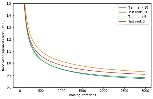
We see that the training error for the rank 5 and rank 10 models are virtually identical, but the test error is lower for the rank 5 model. We can interpret this as the rank 10 model overfitting more, which is often the case for more complex models.
Next, how can we use this model? Well, the rows of the matrix correspond to movies, and the columns of matrix correspond to users. So if we want to know how much user #179 likes movie #2451 (Lord of the Rings: The Fellowship of the Ring), then we compute :
A[2451] @ B[:, 179]Output
4.411312294862265
We see that the expected rating (out of 5) for this user and movie is about 4.41. So we expect that this user will like this movie, and we may choose to recommend it.
But we want to find the best recommendation for this user. To do this we can simply compute the product , which will give a vector with expected rating for every single movie, and then we simply sort. Below we can see the 5 movies with the highest and lowest expected ratings for this user.
import pandas as pd

movies = pd.read_csv(
    os.path.join(DATASET_PATH, "movie_titles.csv"),
    names=["index", "year", "name"],
    usecols=[2],
)
movies["ratings-179"] = A @ B[:, 179]
movies.sort_values("ratings-179", ascending=False)| name | ratings-179 | |
|---|---|---|
| 10755 | Kirby: A Dark & Stormy Knight | 9.645918 |
| 15833 | Paternal Instinct | 7.712654 |
| 15355 | Last Hero In China | 7.689984 |
| 14902 | Warren Miller’s: Ride | 7.624472 |
| 2082 | Blood Alley | 7.317524 |
| … | … | … |
| 463 | The Return of Ruben Blades | -6.037189 |
| 12923 | Where the Red Fern Grows 2 | -6.153577 |
| 7067 | Eric Idle’s Personal Best | -6.441100 |
| 538 | Rumpole of the Bailey: Series 4 | -6.740144 |
| 4331 | Sugar: Howling of Angel | -7.015818 |
Note that the expected ratings are not between 0 and 5, but can take on any value (in particular non-integer ones). This is not necessarily a problem, because we only care about the relative rating of the movies.
To me, all these movies all sound quite obscure. And this makes sense, the model does not take factors such as popularity of the movie into account. It also ignores a lot of other data that we may know about the user, such as their age, gender and location. It ignores when the movie is released, and it doesn’t take into account the dates of all the movie ratings of each user. These are all important factors, that could significantly improve the quality of this the recommendation system.
We could try to modify our matrix completion model to take these factors into account, but it’s not obvious how to do this. There is no need to do this however, we use the matrices , to augment any data we have about the movie and the user. And then we can train a new model on top of this data, to create something even better.
We can think of the movies as lying in a really high-dimensional space, and the matrix maps this space onto a much smaller space. The same is true for the and the ‘space’ of users. We can then use this embedding into a lower dimensional space as the input of another model.
Unfortunately we don’t have access to more information about the users (due to obvious privacy concerns), so this is difficult to demonstrate. But the point is this: the decomposition is both interpretable, and can be used as a building block for more advanced machine learning models.
Conclusion
In summary we have seen that low-rank matrix decompositions have many useful applications in machine learning. They are powerful because they can be learned using relatively little data, and have the ability to complete missing data. Unlike many other machine learning models, computing low-rank matrix decompositions of data can be done quickly.
Even though they come with some limitations, they can always be used as a building block for more advanced machine learning models. This is because they can give an interpretable, low-dimensional representation of very high-dimensional data. We also didn’t even come close to discussing all their applications, or algorithms on how to find and optimize them.
In the next post I will look at a generalization of low-rank matrix decompositions: tensor decompositions. While more complicated, these decompositions are even more powerful at reducing the dimensionality of very high-dimensional data.
Keep reading
10th of March, 2022
We recently made a paper about supervised machine learning using tensors, here's the gist of how this works.
read more →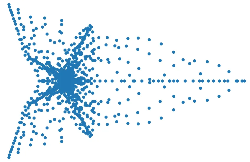
29th of March, 2022
Linear least-squares system pop up everywhere, and there are many fast way to solve them. We'll be looking at one such way: GMRES.
read more →
29th of August, 2021
Parsing and editing Word documents automatically can be extremely useful, but doing it in Python is not that straightforward.
read more →
31st of May, 2021
Finally, let's look at how we can automatically sharpen images, without knowing how they were blurred in the first place.
read more →
2nd of May, 2021
Deconvolving and sharpening images is actually pretty tricky. Let's have a look at some more advanced methods for deconvolution.
read more →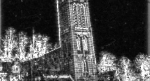
9th of April, 2021
In order to automatically sharpen images, we need to first understand how a computer can judge how 'natural' an image looks.
read more →
13th of March, 2021
Deconvolution is one of the cornerstones of image processing. Let's take a look at how it works.
read more →
15th of January, 2025
I made an array programming language as a language extension to Rust
read more →
1st of August, 2024
Self-hosting your own cloud services not only saves money, it is also a great way to learn
read more →
7th of October, 2023
In my first dive into Rust, I implemented an unscented Kalman filter in and made it 20x faster than the equivalent Python implementation.
read more →
1st of May, 2023
I made an interactive dashboard for this website, and here is the story of how I did it.
read more →
26th of February, 2023
Read this blog post if you're curious what I worked on during my PhD!
read more →
13th of February, 2021
I have 15 years worth of email traffic data, let's take a closer look and discover some fascinating patterns.
read more →
9th of November, 2020
We use exams to determine how much a student knows, but exams aren't perfect. How can we estimate the uncertainty in students' exams scores?
read more →
26th of August, 2020
Cross validation is extremely important, but how should we choose the size of our validation and test sets?
read more →
12th of August, 2020
I use last.fm to track my music listening. Let's look at my data to discover how my musical preferences evolve over time.
read more →
10th of August, 2020
Normally distributed data is great, but how do you know whether your data is normally distributed?
read more →
20th of June, 2020
Judging in figure skating is biased. Let's use data science to figure out just how bad the issue is.
read more →