Modeling uncertainty in exam scores

We widely use exams in education to gauge the level of students. The result of an exam is really only indicator of the students actual level, and has a certainly level of uncertainty. In this article we will try to model the uncertainty in the grades of an exam through a Bayesian model, using the amount of points obtained in each question. Such an analysis may be useful in designing good exams, as in principal this error is something we would wish to minimize.

The data

We will use scores for 8 individual questions of a university math exam. We recorded scores of 100 students. Each question is worth 12 points for a total of 96 points, and students could obtain anywhere between 0 and 12 points for each question.

Notice: this data is modified from the original in multiple ways due to privacy reasons. The modifications preserve most qualitative statistical properties._

Modeling the data

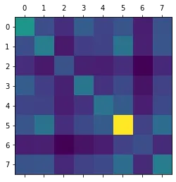
Let $S$ denote the total exam score, and let $G_j$ denote the score obtained for the $j$ th question. Obviously these variables are not independent, high scores in one question are a indicator the student will get high scores in another question as well. For simplicity we want to model the question scores as conditionally independent given the total score $S$ . The idea behind this is that $S$ is an unbiased measurement of the students abilities, and the score obtained for a question should only depend on the student’s abilities. This ignores the fact that some questions test similar aspects of the course, and so are more correlated compared to others. If we plot the covariance matrix of the scores we see that there doesn’t seem to be a strong correlation between question scores. We do however see that the 6th question has a higher variance than the other questions

Now we need to obtain a good model for the conditional probability $P(G_j|S)$ . We will model $G_j$ by a binomial distribution, which corresponds to assuming $G_j$ consists of $12$ ‘subproblems’, of which the student has equal chance of solving. While this does not seem like a natural assumption, it is very convenient. If $m_j$ denotes the total score obtainable for question $G_j$ this gives model

P(G_j|S) \propto P(G_j|p_j,S)P(p_j|S),

with

G_j|p_j,S \sim \mathrm{Bin}(p_j,m_j).

Next we need to model the conditional distribution $P(p_j|S)$ . We tried linear and quadratic regression on $\mathrm{logit}(p_j)$ , but this tends to perform badly near the limits $S=0$ and $S=96$ , and in general tends to shift the predictions towards the global mean. Instead we want a model such that if $S=0$ then $p_j$ is concentrated near zero. To do this we model $p_j$ with a beta distribution, whose parameters depend quadratically on $S$ . More precisely if $\hat S= S/96$ (which supported on $[0,1]$ ), then we set

p_j|S,\alpha_0,\alpha^j_1,\beta^j_0,\beta^j_1 \sim \mathrm{Beta}\left(e^{\alpha^j_0} S+e^{\alpha^j_1} S^2+\tau,\, e^{\beta^j_0} (1-S)+e^{\beta^j_1} (1-S)^2+\tau\right),

where $\tau=0.01$ is a small regularization parameter. This model has $p_j$ constrained close to $0$ if $S$ is small (and similarly $p_j\simeq 1$ if $S$ close to 96), and also has enough flexibility to fit our data reasonably well. The exponentials are used both to force the parameters to be positive, and this parametrization also improves the fit. The parameters $\alpha_i,\beta_i$ are given normal priors with mean $0$ and large sigma, although the fit is not sensitive on this prior.

We will model all the parameters in this model using a Monte Carlo Markov Chain (MCMC) simulation using pymc3. With pymc3 it is very straightforward to implement this model, and requires only a couple lines of code. In the end we obtain samples for the variables $G_j$ , and we can model the error in the total score by looking at the distribution of the posterior $\sum_{j=1}^{8} G_j$ .

Results

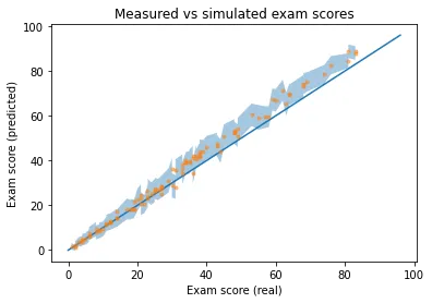
First we compare the distribution of the predicted exam scores to the actual exam scores. The graph below shows the real scores on the horizontal axis, and predicted scores on vertical axis. The vertically shaded area indicates one standard deviation. The model appears to by unbiased for lower scores, but picks up a slight bias for higher scores. In the original unmodified data this behavior was not apparent, and is therefore likely a byproduct of how the data was modified due to privacy concerns.

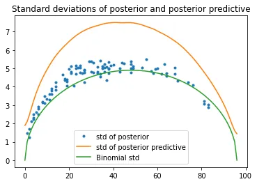
The goal of this project is to simulate the error in the exam score. Below we plot the the standard deviations of the predicted scores as function of total score. We compare this to a theoretical variance coming from a binomial distribution with 96 trials, and we see that the error is close to this theoretical variance. This means that most of the variance in posterior comes directly from the binomial distributions modeling the question scores $G_j$ . We also plot the the variance in the posterior predictive, which is significantly higher. This makes sense, because for the posterior predictive we do not just model the error in each question score, we also have to predict the scores for each question given just the total score.

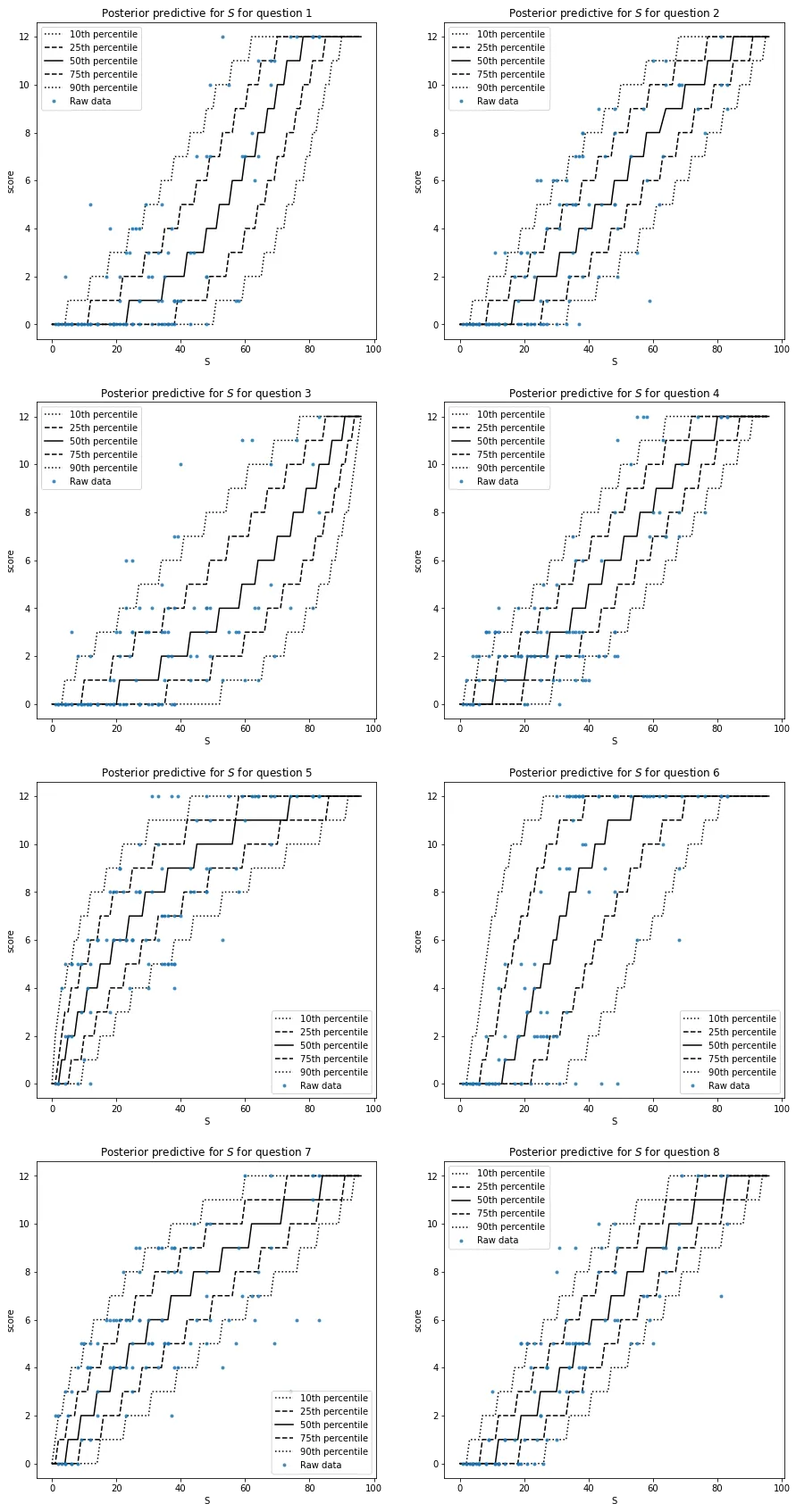
To measure how well our model describes the data, we compare the posterior predictive for each question to the data for each question as function of total score. Here we see that our model describes the distribution quite well for most questions, although in some questions the model underestimates the spread of the data. This is likely because the binomial model is not accurate. To model the questions scores more accurately we would need to step away from the binomial model. However this would make the model more complicated, and the current model does give reasonable predictions for the most part.

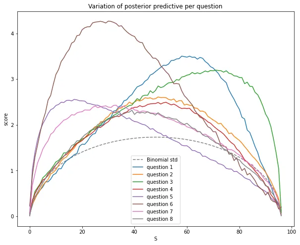
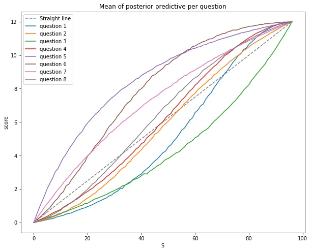
Evaluation the qualities of questions

We can also use the posterior predictive to qualitatively evaluate the quality of questions. Let us plot the standard deviation and mean of the posterior predictive for each individual question as function of the total score $S$ below. In a perfect question the variation is as low as possible, and the mean should be relatively close to the straight line. All in all this means that the question provides as much information about the students abilities. Based on this it seems that questions 2,4,8 are quite good, whereas 1,3,6 are not as good. In particular the points obtained for question 6 has the weakest correlation with the total score. Question 5 seems to have been relatively easy, whereas question 3 appears to have been difficult. Analyzing questions in such a manner can be useful for designing future tests, as well as determining what aspects of the course the students found easier or more difficult.

Keep reading

Time series analysis of my email traffic

13th of February, 2021

I have 15 years worth of email traffic data, let's take a closer look and discover some fascinating patterns.

data-science statistics

How big should my validation set be?

26th of August, 2020

Cross validation is extremely important, but how should we choose the size of our validation and test sets?

data-science statistics

Is my data normal?

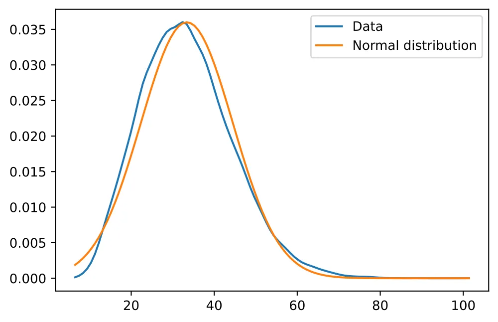
10th of August, 2020

Normally distributed data is great, but how do you know whether your data is normally distributed?

data-science statistics

On Kalman filters and how I made them 20x faster using Rust

7th of October, 2023

In my first dive into Rust, I implemented an unscented Kalman filter in and made it 20x faster than the equivalent Python implementation.

website data-science tools

Dev log: interactive website dashboard

1st of May, 2023

I made an interactive dashboard for this website, and here is the story of how I did it.

website data-science tools

How do my music preferences evolve?

12th of August, 2020

I use last.fm to track my music listening. Let's look at my data to discover how my musical preferences evolve over time.

data-science music

Bias in figure skating judging

20th of June, 2020

Judging in figure skating is biased. Let's use data science to figure out just how bad the issue is.

data-science

Introducing the IJ Programming Language

15th of January, 2025

I made an array programming language as a language extension to Rust

coding

My self-hosting journey

1st of August, 2024

Self-hosting your own cloud services not only saves money, it is also a great way to learn

website tools

My thesis in a nutshell

26th of February, 2023

Read this blog post if you're curious what I worked on during my PhD!

math

GMRES: or how to do fast linear algebra

29th of March, 2022

Linear least-squares system pop up everywhere, and there are many fast way to solve them. We'll be looking at one such way: GMRES.

mathematics linear-algebra code

Machine learning with discretized functions and tensors

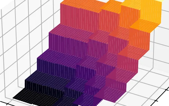
10th of March, 2022

We recently made a paper about supervised machine learning using tensors, here's the gist of how this works.

machine-learning mathematics linear-algebra code

Low-rank matrices: using structure to recover missing data

26th of September, 2021

A lot of data is naturally of 'low rank'. I will explain what this means, and how to exploit this fact.

machine-learning mathematics linear-algebra code

How to edit Microsoft Word documents in Python

29th of August, 2021

Parsing and editing Word documents automatically can be extremely useful, but doing it in Python is not that straightforward.

data-mining code

Blind deconvolution #4: Blind deconvolution

31st of May, 2021

Finally, let's look at how we can automatically sharpen images, without knowing how they were blurred in the first place.

machine-learning computer-vision

Blind Deconvolution #3: More about non-blind deconvolution

2nd of May, 2021

Deconvolving and sharpening images is actually pretty tricky. Let's have a look at some more advanced methods for deconvolution.

machine-learning signal-processing computer-vision

Blind Deconvolution #2: Image Priors

9th of April, 2021

In order to automatically sharpen images, we need to first understand how a computer can judge how 'natural' an image looks.

machine-learning signal-processing computer-vision

Blind Deconvolution #1: Non-blind Deconvolution

13th of March, 2021

Deconvolution is one of the cornerstones of image processing. Let's take a look at how it works.

machine-learning signal-processing computer-vision

First post

19th of June, 2020

My first post in this blog

jekyll