Blind Deconvolution #1: Non-blind Deconvolution

I recently became interested in blind deconvolution. Initially I didn’t even know the proper name for this, I simply wondered if it’s possible to automatically sharpen images given we have some limited information about how they are blurred. Then I went on to do some actual research, and I started diving into the fascinating topic of blind deconvolution. This post will be the first of several, where I dive into blind deconvolution. In the end I will actually look at the implementation of one or two blind deconvolution methods. It turns out blind deconvolution is very difficult and has a vast scope of literature associated to it. Therefore I will split it up into several posts. This is my preliminary plan:

Part I: Introduction to convolution and deconvolution
Part II: Comparing different image priors on a toy problem
Part III: A deep look at blind deconvolution, and implementing it ourselves

Without further ado, let’s figure out what (blind) deconvolution is in the first place!

Blur as convolution

There are many types of blur that can be applied to images, but there are arguably two main types. The first is lens blur, coming from the lens not being perfectly in focus or from imperfections in the optics. And the second is motion blur, which is caused by the camera or the photographed object moving. Both of these types of blur can be described by convolution of the image $x$ with a kernel or point spread function (PSF) $k$ :

(x*k)[i,j] = \sum_{l,m}x[i-l,j-m]k[l,m].

One particular PSF is the delta function, whose only nonzero entry is $\delta[0,0]=1$ . It is the identity operation for convolution:

x*\delta = x.

Often point pread functions have finite support; they are only non-zero for a finite number of entries. In this case we can write the PSF as a matrix, where the middle entry corresponds to $k[0,0]$ . In this case the delta function is a $1\times 1$ matrix with $1$ as it’s only entry.

Box blur

Another very simple (but not necessarily natural) PSF is given by a constant matrix. For example,

k = \frac19\begin{pmatrix}1&1&1\\1&1&1\\1&1&1\end{pmatrix}.

Here we divide by 9 so that the total sum of entries of $k$ is 1. This is useful so that convolution with $k$ preserves the magnitude of $x$ . If not, then the image would become brighter or dimmer after convolution, which we don’t want.

Convolution with a matrix like this has a name; it’s called box blur. It’s a very simple type of blur which replaces each pixel by an average of it’s neighboring pixels. It’s main use is that it’s very fast and easy implement, and to the human eye looks quite a lot like other types of blur.

Gaussian blur

Lens blur can be approximated by a Gaussian PSF, i.e. a kernel $k$ such that

k[i,j] \propto \exp\left(-\frac{i^2+j^2}{2\sigma^2}\right),

for some $\sigma$ . With $\sigma=1$ the magnitude will decay by one standard deviation per pixel. Visually this looks quite similar to box blur, especially for smaller amounts of blur, but Gaussian blur is smoother, and more accurately emulates lens blur.

Motion blur

Motion blur can be described by PSF which, when seen as an image, is a line segment. For example a horizontal line segment through the middle of the PSF is equivalent to camera motion in the horizontal axis. For real life-motion blur this is really only true if the entire scene is equally far away, for example if we consider a spacecraft in orbit taking photos of the Earth’s surface. Otherwise the amount and direction of motion blur is not uniform throughout the image.

Comparison of blur types

We will apply all types of blur to a cropped and scaled image of the St. Vitus church in my hometown taken in 1946 (image credit: Koos Raucamp ).

The first image shows a delta PSF. The top-right shows box blur with a $3\times 3$ box. The bottom-left image shows Gaussian blur, with $\sigma=1$ . Finally the bottom-right image shows motion blur with a top-left to bottom-right diagonal line segment of 5 pixels in length.

Fourier transforms and deconvolution

There is a remarkable relationship between the Fourier transform and convolution, both in the discrete and continuous case. Recall that the discrete Fourier transform (in one dimension) of a signal $f$ of length $N$ is defined by

\mathcal F(f)[k] = \sum_n f[n]\exp\left(\frac{-i2\pi kn}{N}\right).

The Fourier transform turns convolution into (pointwise) multiplication:

\mathcal F(f*g)[k] = \mathcal F(f)[k]\cdot\mathcal F(g)[k].

(This does ignore some issues related to the fact that the signals we consider are not periodic, and we may need to pad the result with zeros and use appropriate normalization. This result is actually very easy to prove, although the details are not important right now.)

This is a very useful property. For one, discrete Fourier transformations can be computed much faster than naively expected using the fast Fourier transform (FFT) algorithm. Naively applying the definition of the discrete Fourier transform to a length $N$ signal requires $O(N^2)$ operations, but the FFT runs in $O(N\log N)$ . It does this by recursively splitting the signal in two; an ‘odd’ and ‘even’ part, and it computes the FFT for both halves and then combines the result to get the FFT of the entire signal. We can use the speed of the FFT to compute the convolution of two length $N$ signals in $O(N\log N)$ as well, simply by doing

f*g = \mathcal F^{-1}(\mathcal F(f)\cdot \mathcal F(g)).

Another thing is that it makes arithmetic with convolution much easier. For example we can use it to deconvolve a signal. That is, we can solve the following problem for $x$ :

y = x*k.

We take the discrete Fourier transform on both sides:

\mathcal F(y) = \mathcal F(x)\cdot \mathcal F(k).

Then we divide and take the inverse discrete Fourier transform to obtain:

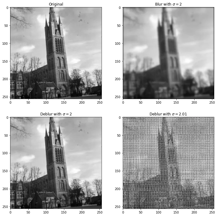
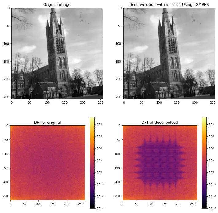
x = \mathcal F^{-1}\left(\frac{\mathcal F(y)}{\mathcal F(k)}\right).

And indeed this works! However, it requires knowing the kernel $k$ exactly. If it is even slightly off, we can get strange results. Below we see an original image in the top left. Then on the top right a version with Gaussian blur with $\sigma=2$ . Then on the bottom we respectively deconvolute with a Gaussian PSF with $\sigma=2$ and $\sigma=2.01$ . The first looks identical to the original image, but then the second doesn’t look similar at all!

What is going on here? A quick look at the discrete Fourier transform of the PSF gives us the answer. Recall that the Fourier transform of a real signal is actually complex, so below we plot the absolute value of the Fourier transform on a logarithmic scale. For reference we also plot the fourier transform of the original and blurred signals.

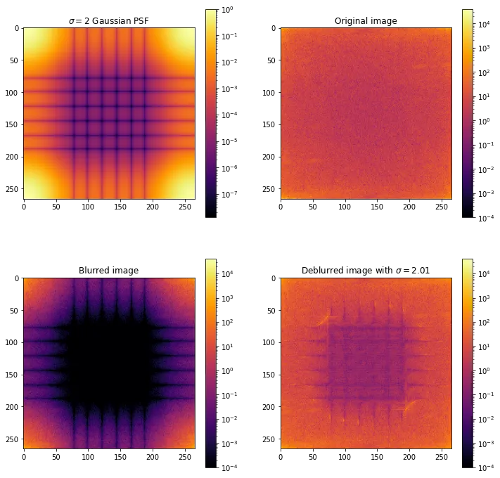
We see that the Fourier transform of the kernel has many values close to $0$ . This means that dividing by such a signal is not numerically stable. Indeed if we slightly perturb either the kernel $k$ or the blurred signal $y$ , we can end up with strange results, as seen above.

Regularizing deconvolution

If we want to do deconvolution, we clearly need something more numerically stable than the naive algorithm of dividing the Fourier-transformed signals. This means putting some kind of regularization that makes the solution look more natural. Above, our main problem is that the Fourier transform of $k$ has values close to zero, so one thing we can try is to add a small number to $\mathcal F(k)$ before division. One problem here is that $\mathcal F(k)$ is complex, so it’s not immediately clear how to add a number to make it nonzero. However, note that we can write

\frac{1}{\mathcal F(k)} = \frac{\mathcal F(k)^*}{\mathcal F(k)\mathcal F(k)^*} = \frac{\mathcal F(k)^*}{|\mathcal F(k)|^2}

In this formula any numerical instability is coming from the the division by $|\mathcal F(k)|^2$ . This is always a positive real number, so we can move it away from zero by adding a constant. This gives us the following formula for deconvolution:

x = \mathcal F\left(\mathcal F(y) \cdot \frac{\mathcal F(k)^*}{|\mathcal F(k)|^2+S}\right)^{-1},

where $S>0$ is a regularization constant. Let’s see how well this works for different values of $S$ :

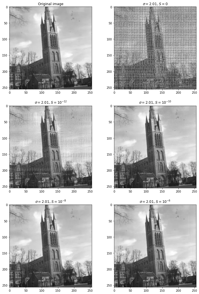
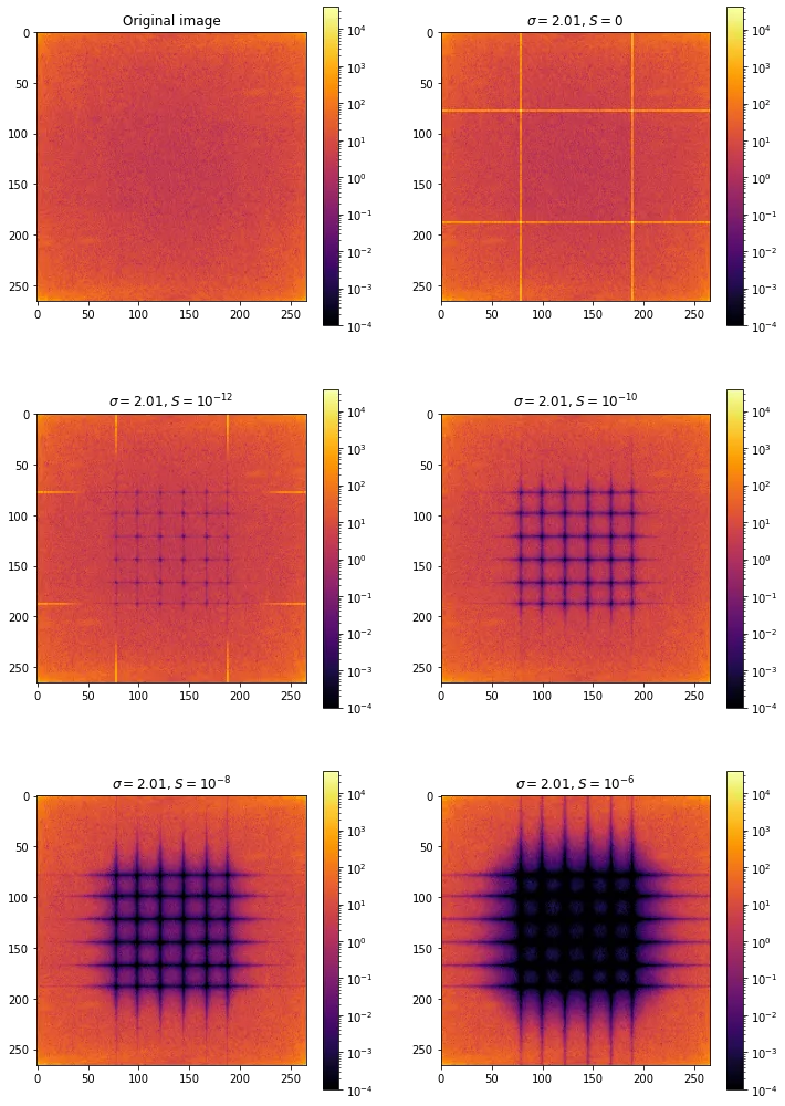
If you look closely, the image looks best for $S=10^{-8}$ . For lower and higher values we see a ringing effect, particularly noticeable in portion of the image occupied by the sky. Visually the best deconvoluted image looks indistinguisble from the original. However if we look at the discrete Fourier transform of the same images, they actually look quite a bit different. (The difference is however exaggerated by the logarithmic scale). There are significant artifacts remaining from the near-zero values of the Fourier transform of the PSF

Deconvolution using linear algebra

Given that I do research in numerical linear algebra, it might be interesting to cast the deconvolution problem into linear algebra. Note that we’re essentially solving the minimization problem

\min_x \|k*x-y\|^2

Since $k*x$ is linear in all the entries of $x$ , we can actually write this as matrix multiplication $k*x = Kx$ , where $K$ is the convolution matrix. For one-dimensional convolution with a kernel $k$ this matrix is $K_{ij} = k[i-j]$ . Using the convolution matrix we can turn deconvolution into a linear least-squares problem, and deconvolution using Fourier transforms gives the exact minimizer of this problem. The reason this exact solution becomes garbage as soon as we slightly perturb $y$ or $k$ is because the matrix $K$ is very ill-conditioned. The condition number of a matrix $K$ tells us how much any numerical errors in a vector $b$ can get amplified if we’re trying to solve the linear system $Kx = b$ .

Fortunately there are ways to deal with ill-conditioned systems through regularization. There are a number of regularization techniques, but in our case this isn’t immediately helpful because of the size of the matrix $K$ . If we consider an $n\times m$ image, then the matrix $K$ is of size $nm\times nm$ . For example if we have a $1024\times 1024$ image then the image requires on the order of 1MB of memory, but the matrix $K$ would take up on the order of 1TB of memory! Obviously that will not fit in the memory of a typical home computer, so working directly with the matrix $K$ is completely infeasible. Moreoever, while the matrix $K$ has a lot of structure, it is not sparse, so we cannot store it as a sparse matrix either.

Nevertheless computing a matrix product $Kx$ is cheap, since it’s just convolution. There are good linear solvers that only need matrix-vector products, without ever forming the matrix explicitly. These are usually iterative Krylov subspace methods. Fortunately scipy has several such solvers, and out of those implemented there it seems that the LGMRES (Loose Generalized Minimal Residual Method) solver works best for this particular problem. Even without regularization this produces decent results. Nevertheless, it’s a bit finicky to get working well, and on my machine the deconvolution takes a full minute, as opposed to a few milliseconds for FFT-based deconvolution.

Conclusion

We can undo blurring caused by convolution if we know the point spread function. Naively performing deconvolution using discrete Fourier transforms is not numerically stable, but we can improve the numerical stability. Nevertheless, unless we know the point-spread function with very high precision, the result is not perfect, as is evident from the Fourier transforms.

In the next part we will start with blind deconvolution. In that case we don’t know the point spread function, so we need to deconvolve with a number of different kernels and iterate towards an approximation of the true PSF. The biggest problem at hand is to have an objective that tells us which deconvolved image ‘looks more natural’. It is not clear a priori what the best way to measure this is, and we will look at several approaches to this problem. Then in the final part we will try one or two algorithms of blind deconvolution.

Keep reading

Blind Deconvolution #3: More about non-blind deconvolution

2nd of May, 2021

Deconvolving and sharpening images is actually pretty tricky. Let's have a look at some more advanced methods for deconvolution.

machine-learning signal-processing computer-vision

Blind Deconvolution #2: Image Priors

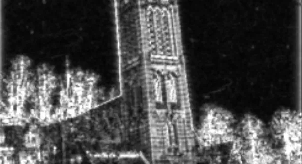
9th of April, 2021

In order to automatically sharpen images, we need to first understand how a computer can judge how 'natural' an image looks.

machine-learning signal-processing computer-vision

Blind deconvolution #4: Blind deconvolution

31st of May, 2021

Finally, let's look at how we can automatically sharpen images, without knowing how they were blurred in the first place.

machine-learning computer-vision

Machine learning with discretized functions and tensors

10th of March, 2022

We recently made a paper about supervised machine learning using tensors, here's the gist of how this works.

machine-learning mathematics linear-algebra code

Low-rank matrices: using structure to recover missing data

26th of September, 2021

A lot of data is naturally of 'low rank'. I will explain what this means, and how to exploit this fact.

machine-learning mathematics linear-algebra code

Introducing the IJ Programming Language

15th of January, 2025

I made an array programming language as a language extension to Rust

coding

My self-hosting journey

1st of August, 2024

Self-hosting your own cloud services not only saves money, it is also a great way to learn

website tools

On Kalman filters and how I made them 20x faster using Rust

7th of October, 2023

In my first dive into Rust, I implemented an unscented Kalman filter in and made it 20x faster than the equivalent Python implementation.

website data-science tools

Dev log: interactive website dashboard

1st of May, 2023

I made an interactive dashboard for this website, and here is the story of how I did it.

website data-science tools

My thesis in a nutshell

26th of February, 2023

Read this blog post if you're curious what I worked on during my PhD!

math

GMRES: or how to do fast linear algebra

29th of March, 2022

Linear least-squares system pop up everywhere, and there are many fast way to solve them. We'll be looking at one such way: GMRES.

mathematics linear-algebra code

How to edit Microsoft Word documents in Python

29th of August, 2021

Parsing and editing Word documents automatically can be extremely useful, but doing it in Python is not that straightforward.

data-mining code

Time series analysis of my email traffic

13th of February, 2021

I have 15 years worth of email traffic data, let's take a closer look and discover some fascinating patterns.

data-science statistics

Modeling uncertainty in exam scores

9th of November, 2020

We use exams to determine how much a student knows, but exams aren't perfect. How can we estimate the uncertainty in students' exams scores?

data-science statistics education

How big should my validation set be?

26th of August, 2020

Cross validation is extremely important, but how should we choose the size of our validation and test sets?

data-science statistics

How do my music preferences evolve?

12th of August, 2020

I use last.fm to track my music listening. Let's look at my data to discover how my musical preferences evolve over time.

data-science music

Is my data normal?

10th of August, 2020

Normally distributed data is great, but how do you know whether your data is normally distributed?

data-science statistics

Bias in figure skating judging

20th of June, 2020

Judging in figure skating is biased. Let's use data science to figure out just how bad the issue is.

data-science

First post

19th of June, 2020

My first post in this blog

jekyll